Isochrone Distance Probabilities
Objectives
In an effort to explore the practicality of isochrones in my research, I’ll be working with calculating the membership probabiltiy of a star within a target galaxy by using the Collins’ method described in this paper.
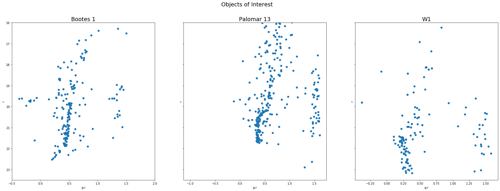
Theres are the following objects I will apply the distance probability method:
Technique
The approach requires a low metallicity isochrone $Z=0.0001$ with a linear age of $10$ gyrs. The .fits for the dataset has a mask that caps the radial velocity error of the DEIMOS targets at $20\text{km/s}$ (ZQUALITY > 2).
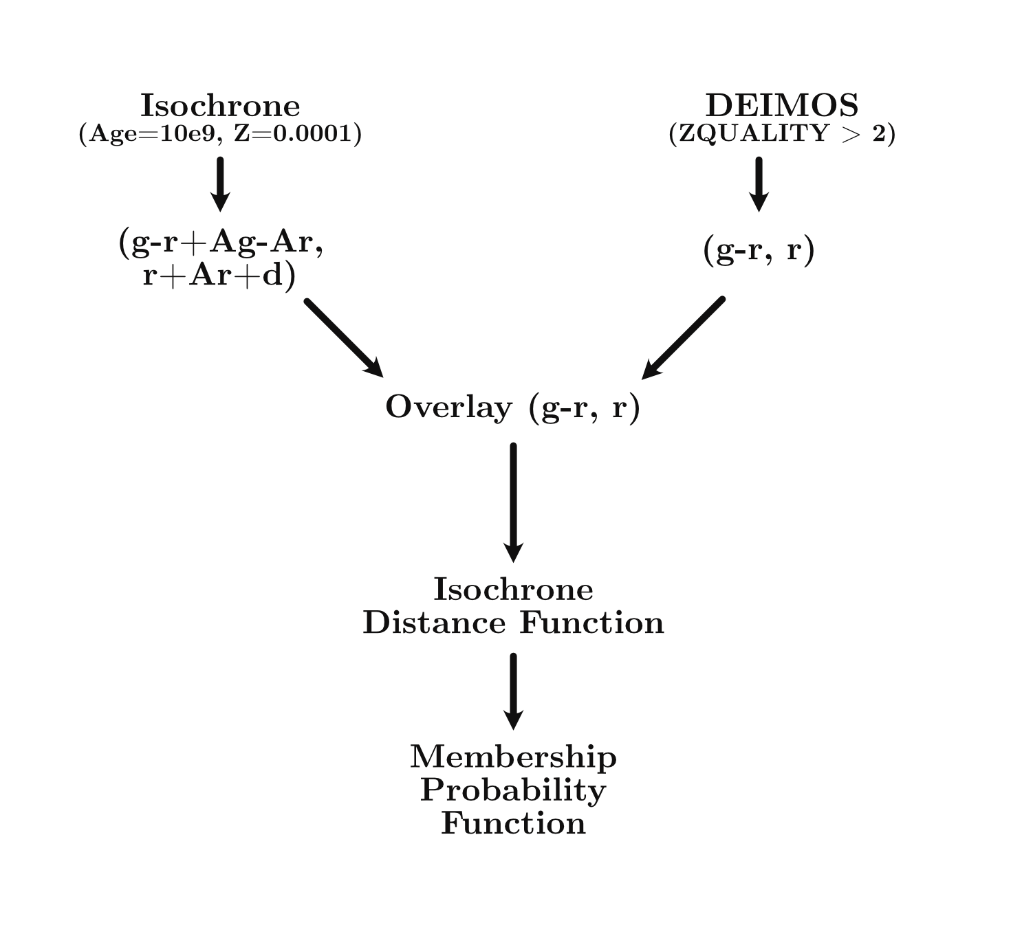
I apply the appropriate corrections using extinction parameters and distance moduli to fit the isochrones. Reference the table below for these values:
| Parameter | Boo1 | Pal13 | Will1 |
|---|---|---|---|
| $A_v$ | 0.04681 | 0.03658 | 0.29698 |
| $A_g$ | 0.0572743 | 0.0447574 | 0.3633694 |
| $A_r$ | 0.0415401 | 0.0324618 | 0.2635458 |
| $E(B-V)$ | 0.0151 | 0.0118 | 0.0958 |
| Distance (kpc) | 66 | 38 | 26 |
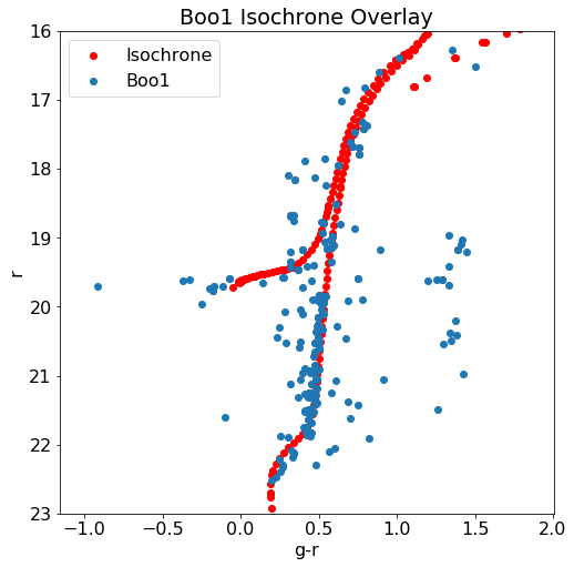
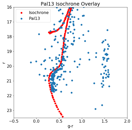
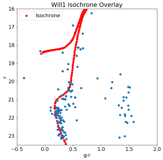
Overplotted Isochrones
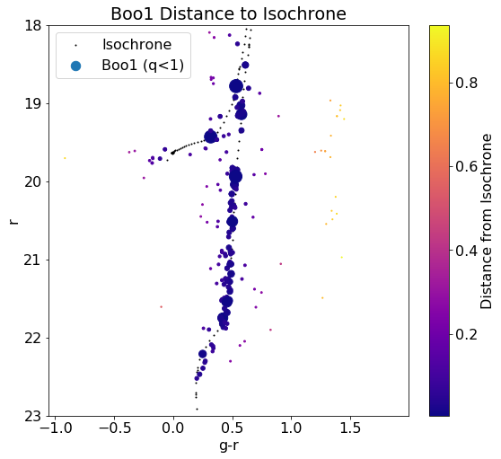
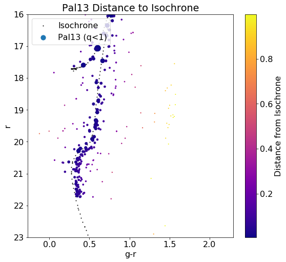
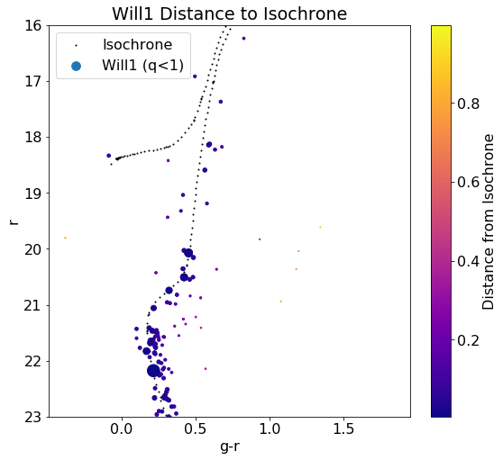
The overplotted isochrones are fitted as shown:
Distance Function
Applying the distance function as discussed in my last post, we receive the following plots (with a distance cut of q $(g-r \times r)$ units):
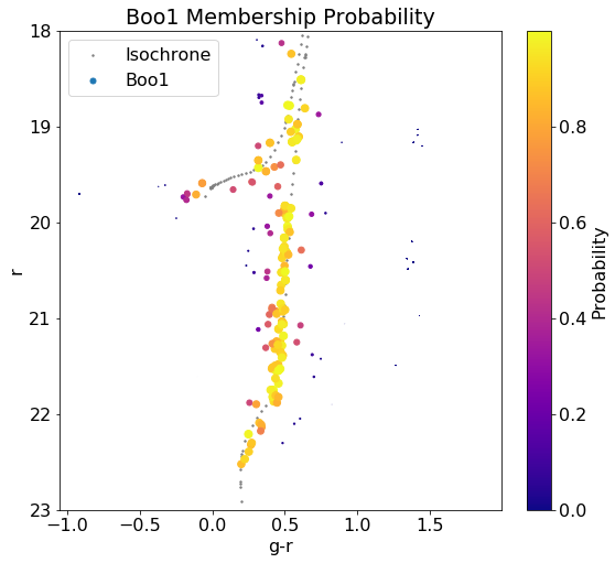
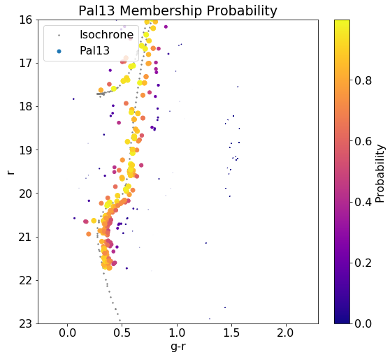
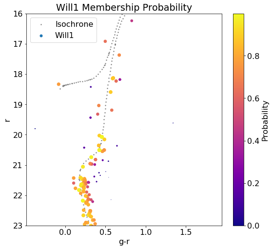
Probability Function
We can feed the values generated from the distance function into a column that uses the Collins’ function for probability. We use $\sigma = 0.1$ as specified by the paper. $d$ is the isochrone distance we feed into the algorithm.
\[P_{\text{CMD}} = \text{exp}(\frac{-d^2_{\text{min}}}{2\sigma^2_{\text{CMD}}})\]We plot the probability overlay: