Working with M67 Isochrones
Objectives
- Figure out how to manipulate isochrone data to fit a color-magnitude diagram.
- Learn how reddening (extinction) and distance affects the location of the isochrone.
- Calculating the distance to isochrone and filtering out candidate stars.
Manipulating isochrone data
Cutting the data
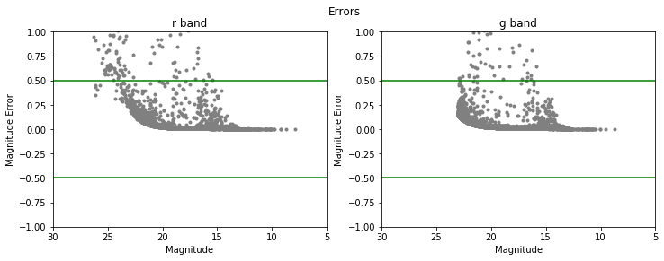
After grabbing the M67 SDSS data, I firstly place bounds on the errors for the $g$ and $r$ bands.
Experimenting with different cut sizes, I plot the following diagrams:
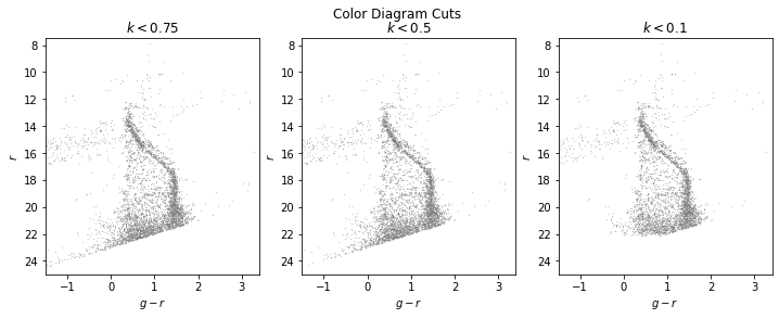
Id decided that I will set these cuts at $|\text{band}_{error}|<0.5$ given that it seems to include an appropriate amount of stars without
over or undercutting the population.
Fitting the isochrone
I downloaded the isochrones using the SDSS ugriz photometric system from here. I used a linear age of about $4\times 10^{9} \text{yr}$ and a metal fraction of $Z \approx 0.0159$ where I deduced from a metallicity of $\text{[Fe/H] = -0.1}$ by $\text{[Fe/H]} = \log_{10} \frac{Z}{0.02}$.
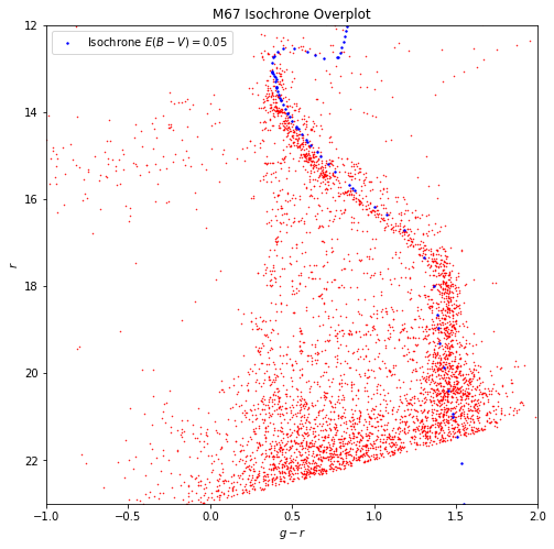
In order to plot the isochrone, I need to fit it against the CMD quite snuggly. This step requires knowledge of the distance modulus (to obtain how much the distance reduces the magnitude of the isochrone) and the reddening/extinction ($E(B-V)$) from the interstellar medium.
The distance to M67 is $d \approx 827.8238 \text{pc}$ and we get extinction values of $A_{g} = 3.793 \times E(B-V)$ and $A_{r} = 2.751 \times E(B-V)$.
We can deduce that
\[M_{r} = r_{iso} + A_{r} + 5\log_{10}{d} - 5 \\ M_{g-r} = g_{iso} - r_{iso} + (A_{g} - A_{r})\]We are not given the actual extinction value, so we’ll use it as a free parameter and vary it until it fits. I found that the value of $E(B-V) \approx 0.05$ works well with this CMD.
Age and Metallicity
To better understand the role of metallicity and age in the context of isochrone plots, I altered the metallicity and age of the isochrone and overplotted them.
By increasing the age from $4\times 10^9$ to $7\times 10^9$:
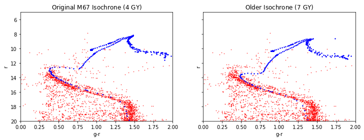
This plot is consistent with the theory that as groups of stars get older, their turn-off point from the main sequence gets lower.
By increasing the metallicity from $Z = 0.0159$ to $Z = 0.03$:
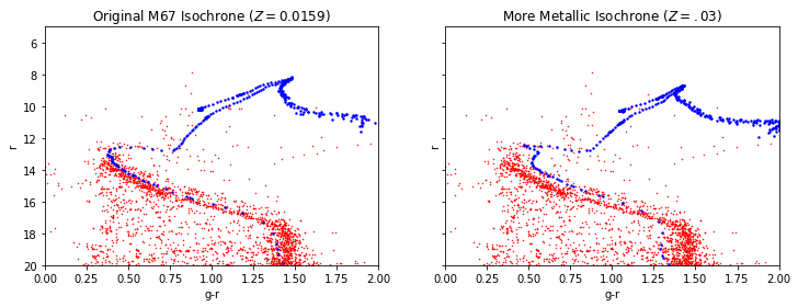
This plot is consistent with the theory that as stars in a CMD have higher metallicites, they shift closer to the red end of the spectrum.
Calculating the Distance to an Isochrone
The goal of the project is to predict star membership based on a variety of factors, one of which is based on the distance a star is to its model isochrone.
I simply iterate over each star in the CMD, then iterate over each isochrone point (I’m guessing a computational complexity of $O(n^2)$) and collecting the distance of each isochrone point to a star, then returning the minimum distance into another array that collects all the minimum distances to the isochrone of each star.
The distance computation is simply geometric (for $k$ stars):
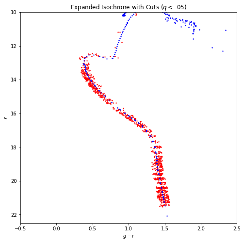
\[\Delta_{g-r} = M_{g-r} - (g_{i} - r_{i})\\ \Delta_{r} = M_{r} - r_{i}\\ \oplus_{i=1}^{i=k} d_{min} = \sqrt{\Delta_{g-r}^2 + \Delta_{r}^2}\]Here is a plot of the CMD with various isochrone distance cuts:
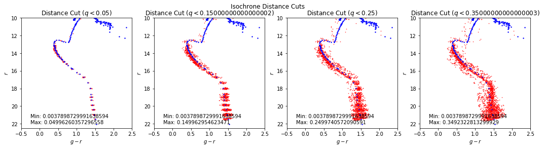
We see that there are ovals surrounding each isochrone point (really just circles that have been squished due to the axes). We can attempt to ameliorate these plots by interpolating the isochrone points by doubling them to increase accuracy within the actual projected isochrone line.
By simply taking the midpoint formula across gr-r space, we can construct additional isochrone points which we can apply the distance function to and get a better resolution. Although it is not perfect and still very much a work in progress, the end result is satisfactory (compared to the first CMD plot in the last figure with the same q cut):